01 – Understanding and Measuring Fatigue
1.1 – Fatigue measurement in subsea power cables
Static sub-sea power cables which undergo repeated strains during use are prone to failure through fatigue. Repeated cyclic loading of elements within the structure of the cable encourages crack nucleation and growth to a point where failure can occur. The main weak point is the lead sheath where cracks allow water ingress leading to tree formation and ultimately electrical failure. In both dynamic cables and static cables, the conductor materials and armour wires can also be damaged by the same fatigue mechanisms
The optical fibre which is embedded in the cable structure is also strained during cyclic loading of the cable, and DAS can be used to measure and track this strain. If the relationship between the strain of the cable elements and the fibre can be determined, fatigue damage can be tracked. With a short measurement (1 week or so) the remaining lifetime of the cable can be estimated, but with a permanent DAS installation the remaining lifetime of the cable can be directly measured.
We recently collected data from a sub-sea export cable which shows two sections of cable at the CPS and J-tube which are subject to cyclic loading above the fatigue limit (the only parts of the cable to be so).
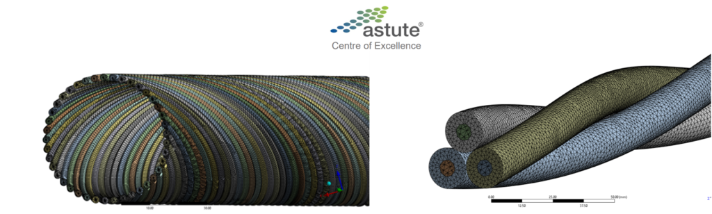
We have partnered with the Astute Centre of Excellence at Swansea University to use finite element analysis of cable structures to determine the remaining lifetime of the cables at these locations so that advice on the necessity of intervention can be given. Thanks to Fawzi Belblidia and the team.
Key takeaways: fatigue and remaining lifetime can be directly measured. This is going to be critical for floating wind but on static cables that are exposed to vibration it is essential knowledge.
1.2 – Designing for Fatigue Resistance
Floating wind is struggling with a lack of solid reference points and standards for design for fatigue.
As the need grows for utilisation of offshore wind, the turbine locations are becoming increasingly diverse and challenging. Floating offshore wind in deeper waters, for example, where the turbines are mounted on floating structures with inter-array cables that may need to suspended above the seabed, leads to increased uncertainty in cable reliability. Indeximate recently attended the Renewable UK Floating Offshore Wind conference in Aberdeen where there were several presentations and discussions on modelling the consequences of suspending cables on their reliability and susceptibility to fatigue, etc. But how do we validate these models and assess cable performance in real life environments? This is an open question but Indeximate has the tools to extract this key info.
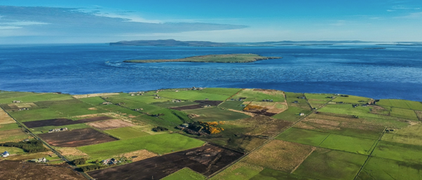
An interesting case study for fatigue resistance comes from our experiences with tidal stream where exposed cables are subject to daily heightened vibration. We have been working with the SAE Renewables MeyGen tidal array off the North coast of Scotland, the largest planned tidal stream project in the world.
MeyGen were aware of the danger that the tidal stream would present to their cables so insisted on quad-armoured cables which are extremely stiff and well-protected from abrasion and have the added advantage of extra weight, which helps to restrict movement and minimise fatigue. Using an ASN DAS system, MeyGen have instrumented the whole of the tidal array cable network and Indeximate have been processing their data to assess the longer-term effects of this harsh environment.
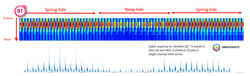
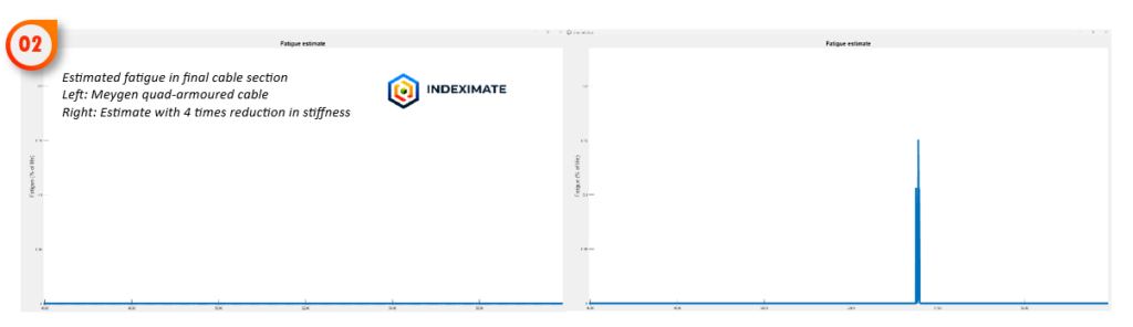
Looking at the vibration of one of the cables in the array over a three-week period in May 2023 (1), we can see very clearly that some sections subject to high levels of vibration, arising from tidal flow – four times a day every day.
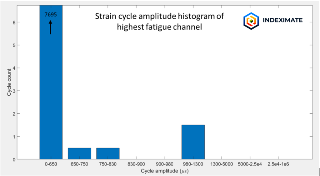
But how much strain is the cable subject to and how do we assess the likely impact of this? We’ve shown previously how we use DAS to measure cable fatigue. In MeyGen’s case the stiffness in the quad-armoured cable restricts the strain on the cable and the measured strain is below the fatigue limit, so we don’t see any indication that the movement is enough to cause significant fatigue. However, if we were to reduce the stiffness by a factor of 4 as would be the case for a single armoured cable, so more strain is transferred to the cable, we can repeat the calculation and see that some of the strain cycle amplitudes could be over the minimum level for fatigue to occur and so fatigue would be observed (2).
Further work is required to refine the strain response and strain-fatigue relationship for different cable types and Indeximate is working with the ASTUTE Centre of Excellence at Swansea University to assess the relationship between the level of strain seen on the fibre and that of the surrounding cable. In addition, practical measurements to assess the response of embedded fibres to cable tension is planned at the OREC Dynamic Cable Test rig.
2.0 – Getting the most out of your data
2.1 – The response of cables to the pressure of tidal flow
Exposure is a big topic for subsea cables, and one of the mechanisms which can de-bury cables is erosion of the sediment by tidal streams. The streams tend to wander in an unpredictable way, and it is important to track this movement over time. We know that the fibres within a power cable are incredibly sensitive to strain, and the pressure that the cable experiences due to changes in the surrounding environment cause changes in strain on the fibre which can be measured. This can still be done on a buried cable which provides an indicator of things to come.
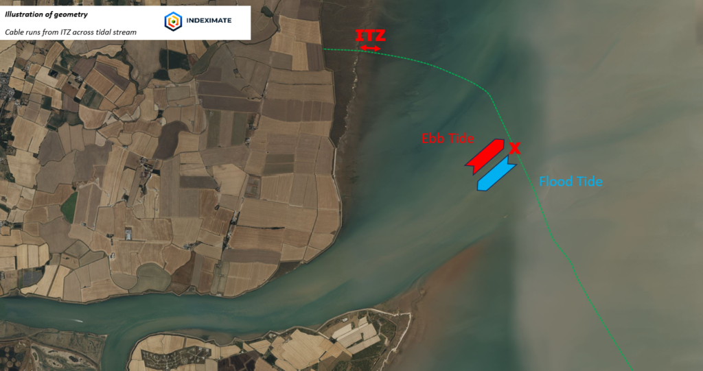
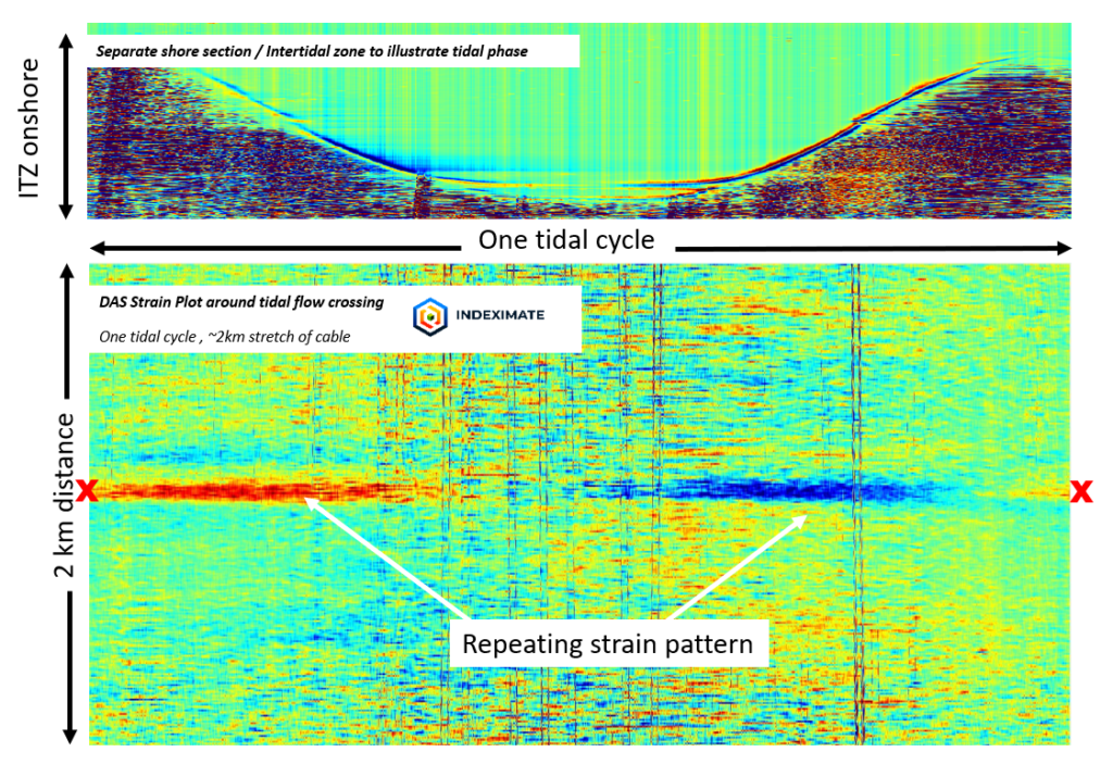
Identifying a tidal stream in an exposed cable is easy – look during the flow and you’ll see noise – job done. In buried sections it’s harder. Careful analysis of DAS data from long recordings from fully buried cables reveals low frequency signals showing tidal related patterns on subsea sections emerging from the noise. DTS analysis shows no equivalent temperature changes in these regions, and we can therefore conclude the cause to be strain. The origin of this strain is from the changes in water pressure as water flows around bathymetric features in the seascape. The image is showing the resultant strain along 2km of fibre where one clear location shows a positive on the ebb tide and negative on the flood tide (the fibre’s core response to increasing pressure is negative). These measurable signals allow tracking of the streams over time, including the sudden changes that may occur in the aftermath of a storm. Not only can the potential erosion location be tracked, but the DAS data can reveal if and when the cable actually becomes exposed. The second image shows an explanation of the bathymetry and what is being affected by the tidal stream.
2.2 – Wind Turbine Structural Health Monitoring
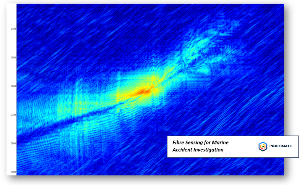
Although we are focussed on cable health monitoring, our Indeximation approach allows us to retain long term data, without losing useful information. This presents opportunities for further analysis and data re-use for lots of additional purposes. For example, Wave height measurement or Marine accident investigation.
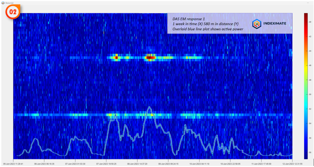
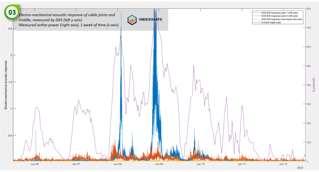
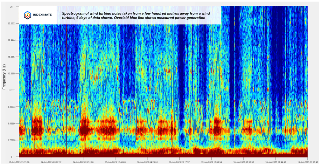
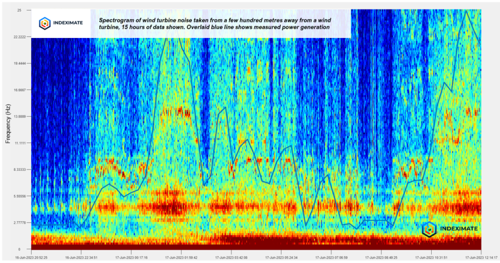
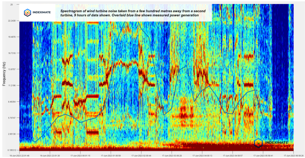
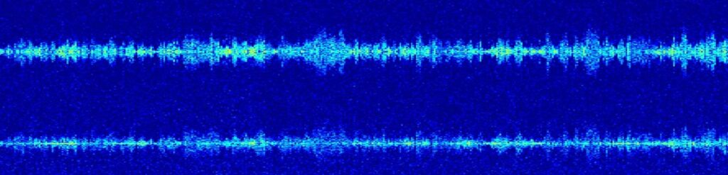
Where the fibre runs through a wind farm, either via the export or inter-array cables, and passes close to or through wind turbines we can take a detailed look at their acoustic properties. The spectrograms below show frequencies below 25 Hz and are taken from an export cable where the fibre passes close to two different wind turbines. The blue line shows the measured power over the period. We expect to see frequencies related to the vibrational modes of the wind turbine towers, which should be relatively stable with time; the strong signals at around 4 Hz in the images below are probably examples of this. Changes or anomalies in these signals could be indicators of structural problems or loose bolts (as explored in this paper – https://link.springer.com/article/10.1007/s13349-021-00483-y). In addition, we can see frequencies that vary with the measured power (image 3), which are probably related to the gearboxes in the turbines.
As we are recording continuously, we build up a huge data store that can either inform on any potential developing problems or allow retrospective analysis after problems occur to give further insight into the causes of failure.
2.2 – Should I choose Quant or Qualitative DAS?
In our work we often get asked by customers about the two different types of DAS unit commonly found and which they should use. As it’s our tool of choice for extracting info on the condition of cables, we thought it was time to put together some of our thoughts on the topic.
You can read the complete long-form article here
3.0 – Identifying artefacts in the acoustic record
3.1 – Forensics for Marine Accident Investigation
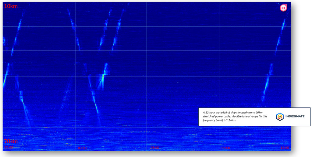
When working on offshore power cables we may be spending our time looking inwards at the cable and the environment but we also by circumstance look outwards at the same time, capturing everything that is taking place in the locality. Ships are a regular occurrence of course and can be of interest to the cable owner due to the potential for damage from bottom trawl or anchoring. We profile the pattern of life and advise on risk.
We also capture information about benign movement on the surface and here there is a great forensic utility for marine accident investigation.
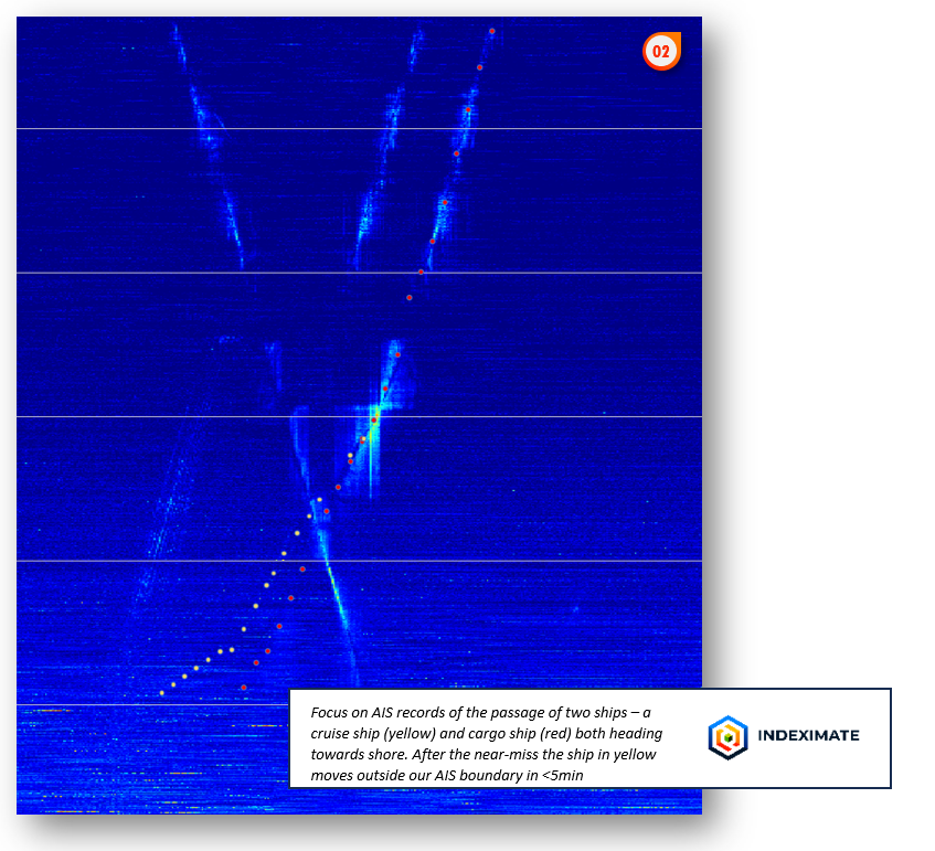
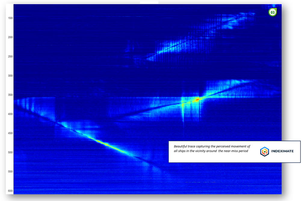
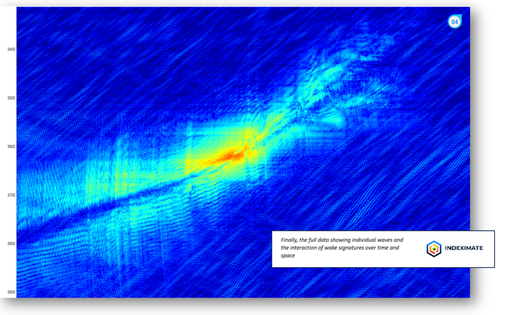
We are used to seeing vessels passing and their wakes incoming, but this pattern (1) caught our eye – a massive pulse in acoustic energy at 4AM that spanned 15km. Looking at our parallel AIS data (2) we can see there are two ships on a crossing trajectory. When we zoom (3) we see the characteristic wake signature with broadside null that cables generally experience, zooming in further (4) we can see the evidence of the wakes interacting over a few minutes.
DAS analysis places the vessels within 90m of each other, AIS tells us the ships are 4kT and 15kT – which should by maritime law keep apart 0.5 nautical miles – a reportable event.
DAS can fill in the gaps in the AIS record, giving a second by second plot of trajectory and position as well as providing evidence on the scale of any event potentially extending the utility of measurement and bringing benefit to asset owners.
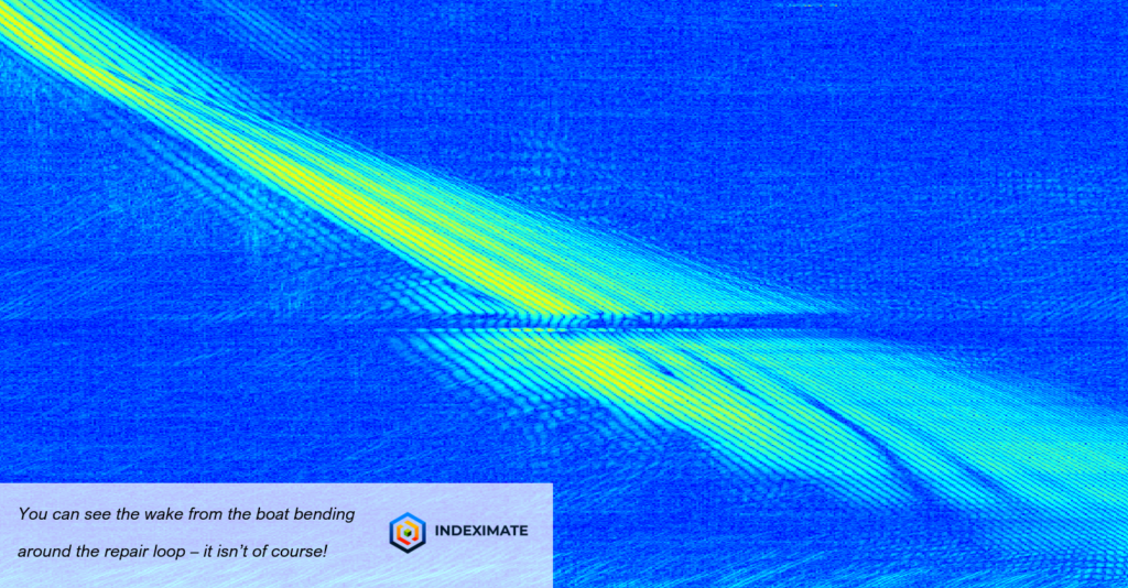
3.2 – Identification of subsea cable repairs
When detecting and measuring electrical and mechanical anomalies it’s good practice to tie up measurements with what you expect to find on the seabed. In the case where you find two points of electrical degradation separated by a few hundred metres of quite differently behaving cable, it’s quite often the case that you are looking at a spliced in additional section of cable – but how to verify?
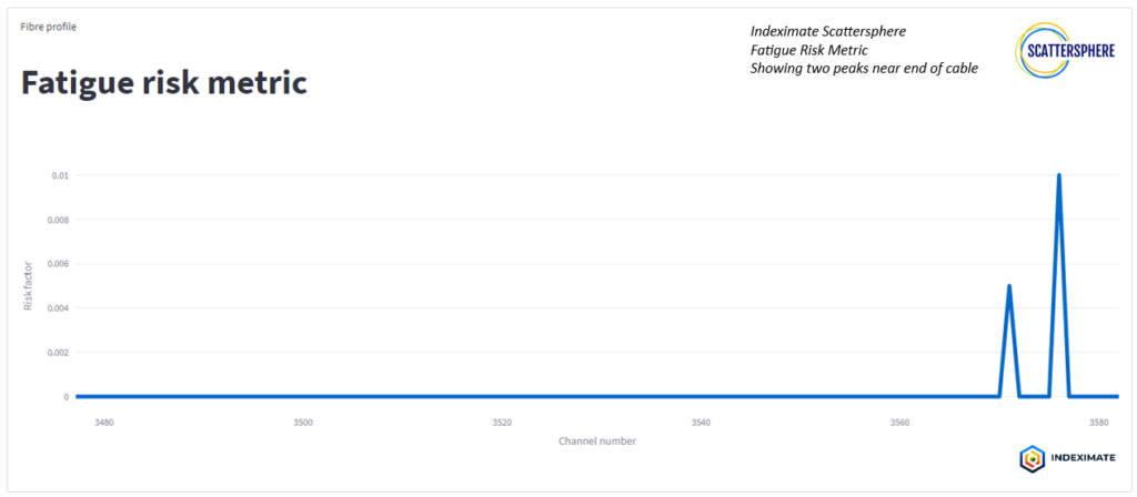
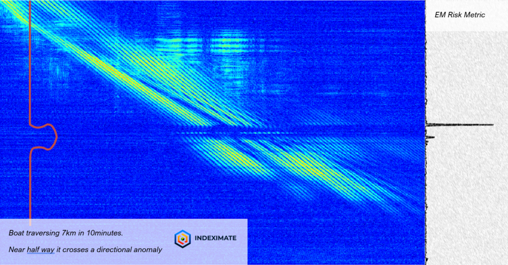
The same instruments we use to measure degradation will also give us the answers. Look at the example below – our EM Risk metric shows two peaks separated by about 250m – classic splice in repair – with one peak here behaving rather poorly compared to the other.
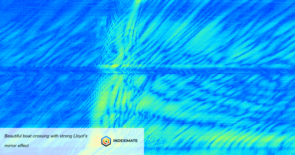
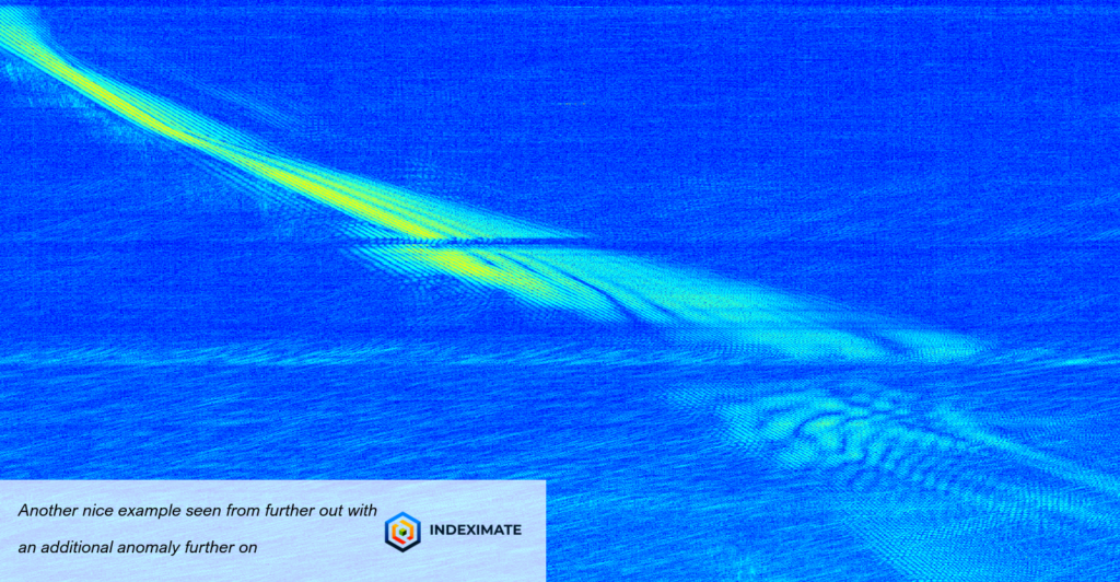
Lots of sound sources exist to help us here – passing boats or the waves themselves – our cables are acoustically directional with sensitivity perpendicular to the cable being much less than along the cable. As the cable turns in a classic “Omega” loop it changes direction by 90° twice – we expect to see a null, a peak and a null before normal service is resumed. As well as exhibiting very nice Lloyd’s mirror effects from the underwater acoustics, the traces can tell us a lot about the routing of cable on the seabed.
3.3 – Measurement of Wave Height
We posted last week on forensic analysis of ship near misses, this week we continue with a nautical theme and explore the Measurement of Wave Height
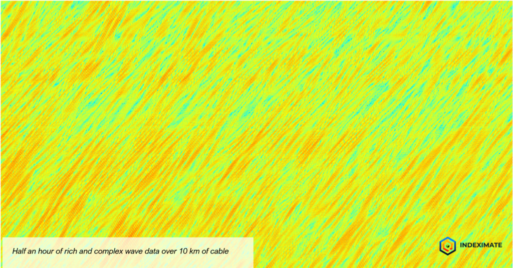
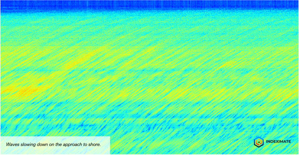
As we’ve shown clearly before, not only are the cables sensitive to sound propagating through the water, but they are sensitive to gravity waves on the sea surface. This is shown by the visibility of ships wakes travelling for 10’s of kilometers along the cable. At the same time, waves generated by wind are clear, and their propagation speed is seen to decrease with depth exactly as expected. What is the mechanism for DAS to be able to detect these waves, and how can this information be used?
The hydrostatic water pressure at the seabed is dependent on the depth of water at that location, and the pressure below the crest of a wave is therefore higher than below the trough. So, as waves pass over the cable, we expect an oscillation in the hydrostatic pressure around the cable. The magnitude of this pressure change depends on a number of well understood factors. The fibre changes length with change in pressure, so this pressure oscillation becomes visible as a signal using DAS. Because the sensitivity of the cable to pressure can be independently measured, the height of the waves can be calculated.
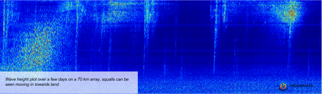
So now, we have a distributed wave height sensor along the whole length of the asset. This array is active all this time, measuring and recording the height and period of every wave along its whole length in real time and with great sensitivity. So, as well as identifying ships from their wake, this information can be used during operations work to monitor for deteriorating weather conditions, as well as studying the environmental conditions along vast tracts of the sea.
Imagine having a wave measuring device at every point in your wind farm.
4.0 – The Thermal & Electrical behaviour of cables
4.1 – Subsea power cable temperature from multiple sources
This week in our series of posts from the end of a cable, we want to highlight the importance and utility of temperature analysis in the case of a power cable crossing other cables & pipelines.
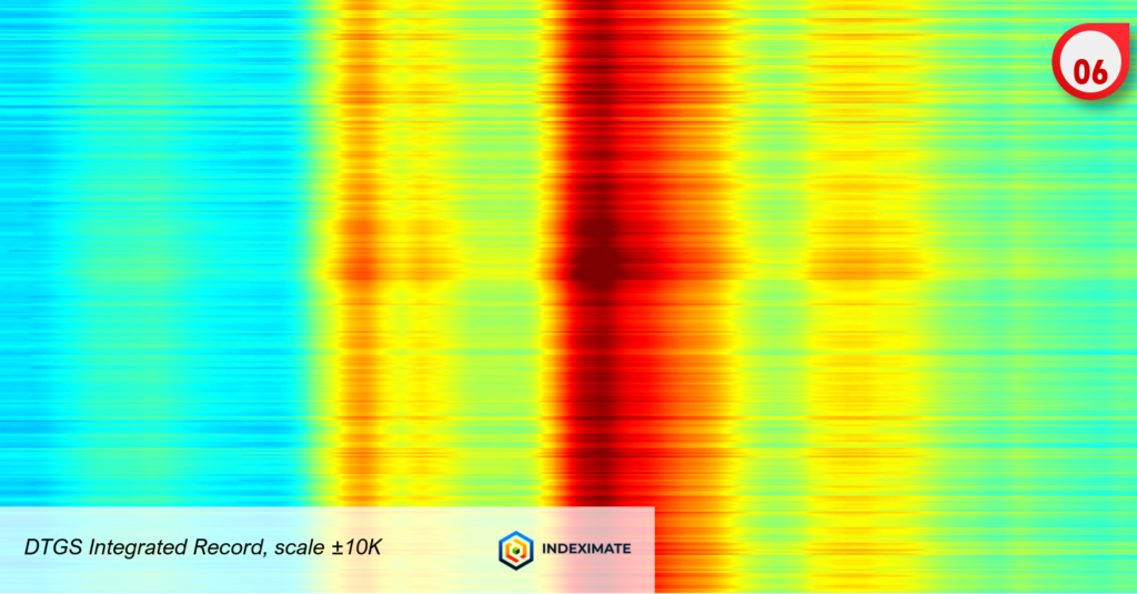
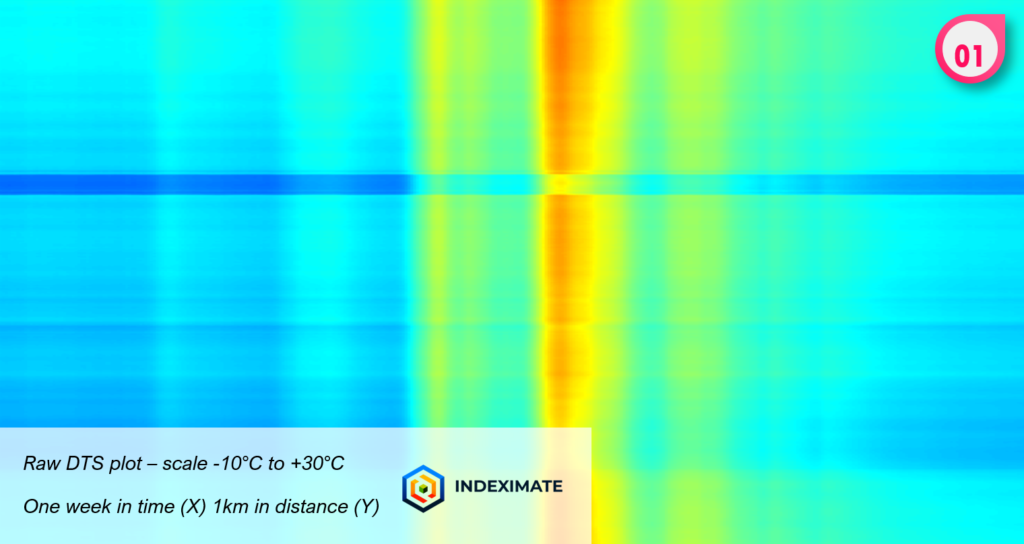
DTS (1) is well established as a tool for identifying hot spots and monitoring thermal ratings. Calibration and attenuation issues can obscure some detail, however when considered as a gradient rather than an absolute and compared with its DAS sibling (DTGS) the picture becomes richer and calibration issues can be resolved.
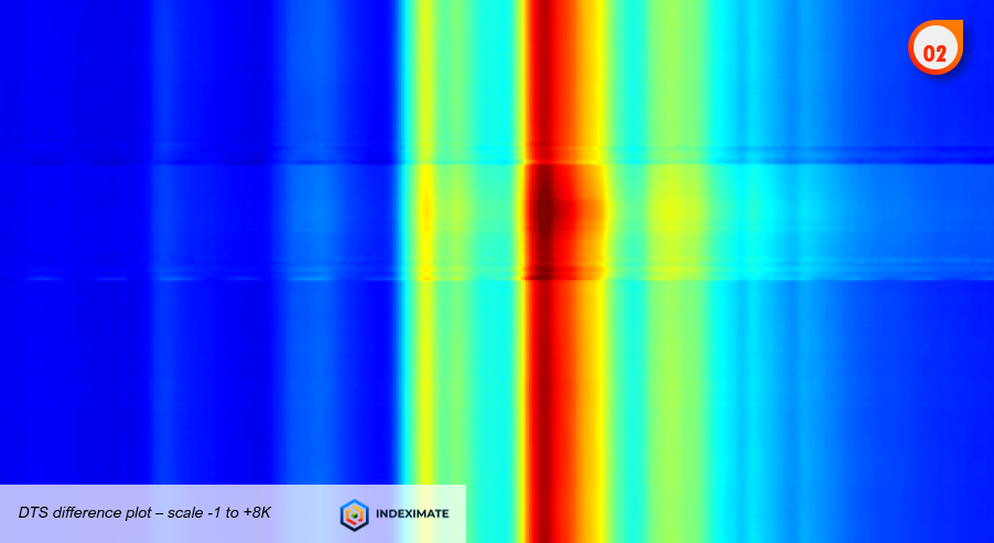
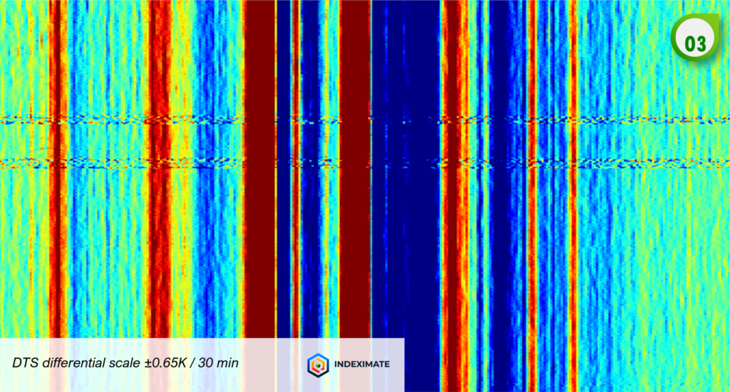
The same DTS plotted as a delta (2) from a one-week period after day zero shows a temperature rise in-line with wind related production and on a vertical scale of 1km shows a clear disturbed region around a cable & pipeline crossing –often treated with mattressing or rock dumping. Plotted as rate of change (3) it shows two strong heating periods with a peak heating rate of 0.1K per 30min and the crossings become very clear.
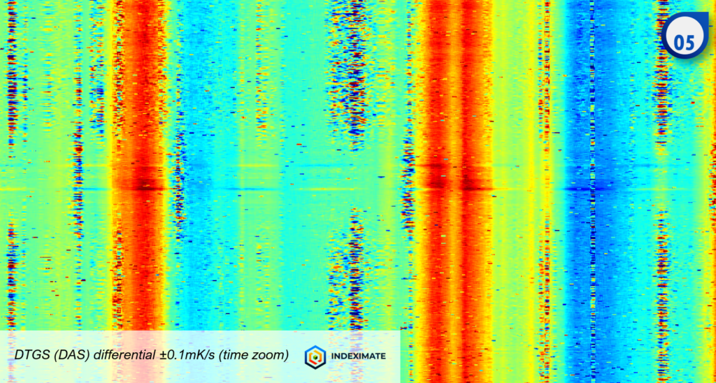
DAS (in its DTGS guise) adds further nuance (4) here the scale is in ±0.1mK/s! The pictures are broadly similar but if we zoom in time (5) we see very nuanced heating and cooling. Finally if we integrate the DTGS to pull out TOTAL change we recover a perspective similar to the DTS delta plot but with added fine detail of fine scale environment change on top of the forced heating (6).
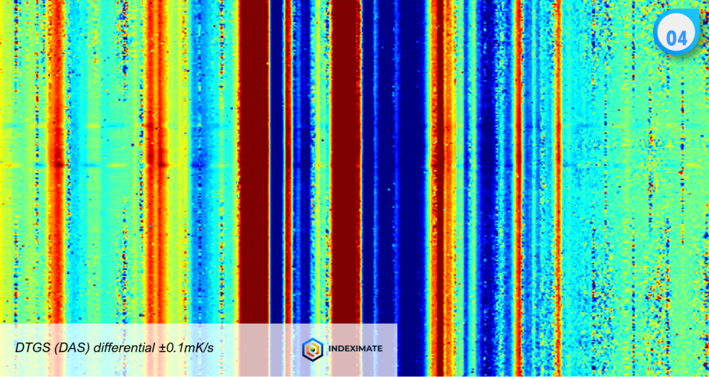
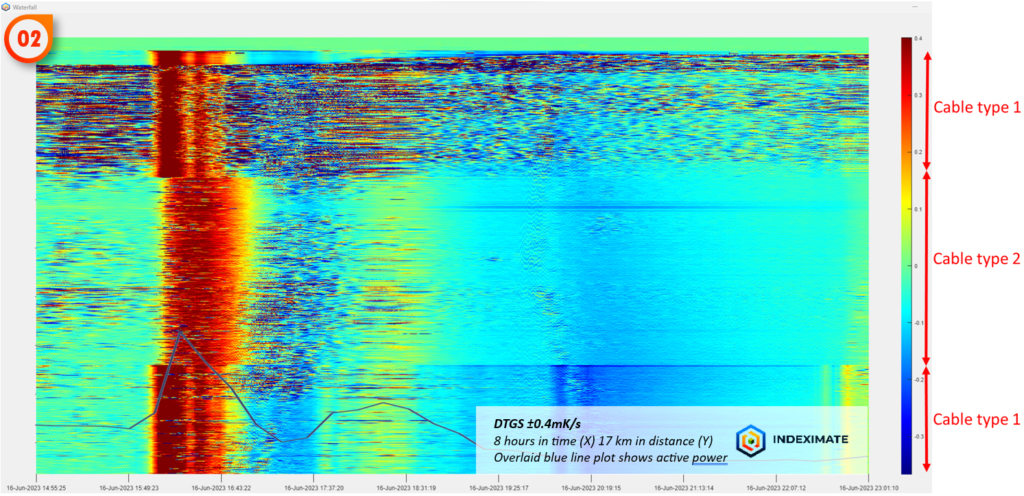
4.2 – Exploring the response to power
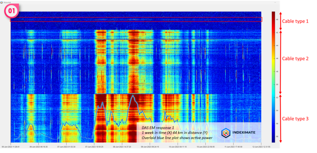
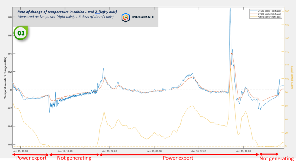
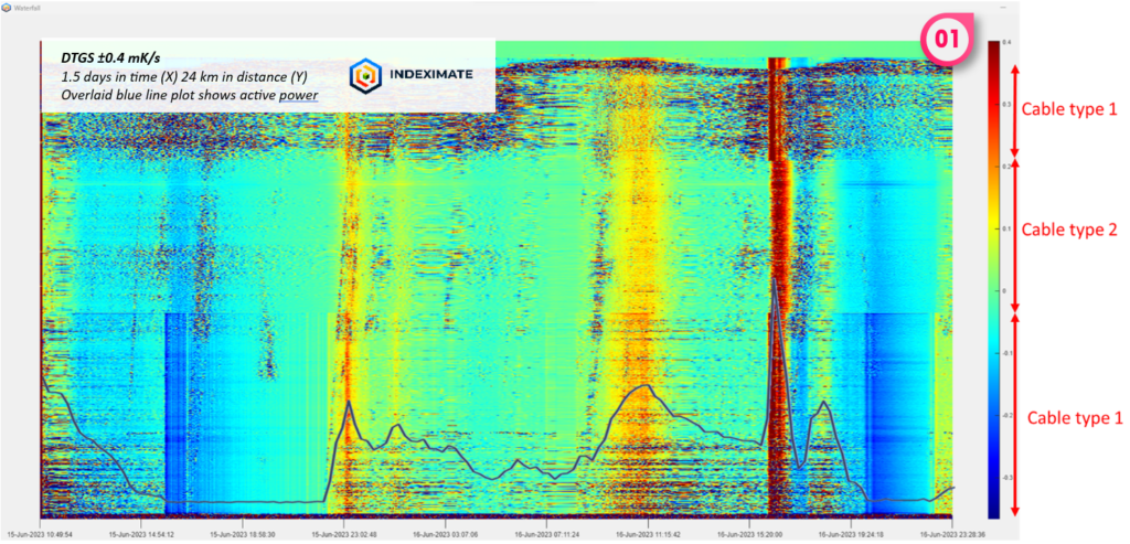
We’ve previously shown how the thermal response of subsea cables reveals important information about the properties and condition of the cables. Due to its remarkable sensitivity to temperature, DAS provides valuable insight into heating from wind power generation. The Distributed Temperature Gradient Sensing (DTGS: heating rate – not absolute temperature) images (1 and 2) show how the thermal response to current varies in two different cable sections. Cable 2 shows a retarded heating cycle due to increased insulation around the fibre. The blue overlay shows the measured power generation.
Plotting each section as a time series (3) verifies that the output closely follows the measured active power from the wind farm when generating.
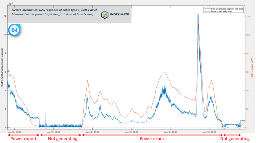
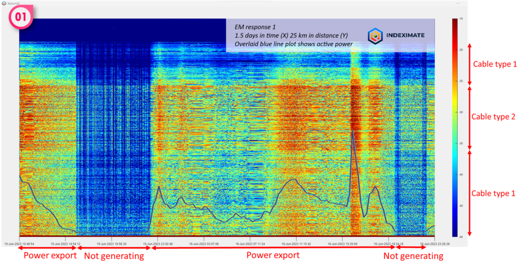
We also look at the electro-mechanical response at every point along the cable (4). As expected, we see a very clear relationship to generated power. This electro-mechanical response is however also affected by cable integrity, we use this to derive weakness metrics at every point along the cable, something we will explore further in the next post.
4.3 – Introducing the EM metrics
We introduced above how the electro-mechanical response of a cable to applied electrical power reveals key information about the condition and properties of the cable.
We derive two indicators from the acoustic response, each of which reveals different information about integrity. The first indicator (EM1) is related to the mechanical properties of the cable, such as weakness in the armour or deformation. The second indicator (EM2) is a direct result of the cable response to applied current. Image (1) illustrates EM1 from an export cable and shows how it matches over time with measured power (overlaid blue line). There are two cable types present and the difference between them is very clear.
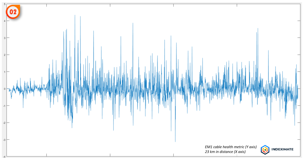
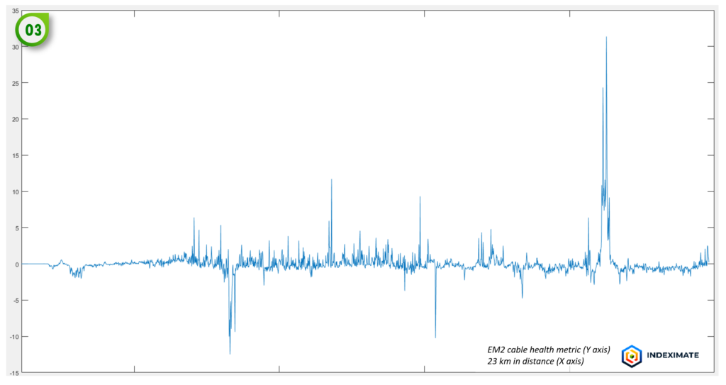
From this response we can derive a metric to indicate areas of weakness or damage. In this case (a healthy cable) for EM1 we see that the performance is relatively consistent (2). EM2, however, shows some clear anomalous locations (3).
EM2 is sensitive to features such as cable and gas pipeline crossings and most of the features we see in the images below can be explained by benign factors. This isn’t always the case, however and we’ll see in our next post what can happen when deterioration arises and how we identify the location of poorly performing sections of cable.
4.4 – Identifying and monitoring suspect sections of cable
Back on the 8th August we introduced how the electro-mechanical response of a cable to applied electrical power reveals key information about the condition and properties of the cable.
We derive two indicators from the acoustic response, each of which reveals different information about integrity. The first indicator (EM1) is related to the mechanical properties of the cable, such as weakness in the armour or deformation. The second indicator (EM2) is a direct result of the cable response to applied current. Image (1) illustrates EM1 from an export cable and shows how it matches over time with measured power (overlaid blue line). There are two cable types present and the difference between them is very clear.
From this response we can derive a metric to indicate areas of weakness or damage. In this case (a healthy cable) for EM1 we see that the performance is relatively consistent (2). EM2, however, shows some clear anomalous locations (3).
EM2 is sensitive to features such as cable and gas pipeline crossings and most of the features we see in the images below can be explained by benign factors. This isn’t always the case, however and we’ll see in our next post what can happen when deterioration arises and how we identify the location of poorly performing sections of cable.